User Guide

A complete guide to working with your data in ISLdata.

ISLdata is a data management system designed for field research. It connects data collection (via ODK or manual import), data organization, and reporting in a single workspace. This guide covers everything you need to know as a day-to-day user of the system.

When you log in, you'll arrive at the Data Viewer — the main interface where you interact with all of your data. The Data Viewer is organized around four core concepts:

Concept	What It Is
Sources	Collections of raw data — synced automatically from ODK Central or ESRI Survey123, imported from spreadsheets, or entered manually. Each source is a table of records with defined fields.
Views	Custom windows into your data. A view can pull from a single source or join multiple sources together, showing only the fields you choose in the order you want.
Dashboards	Visual summaries that combine charts and data widgets on a single page. Useful for monitoring data collection progress or key metrics.
Reports	Structured documents that combine narrative text, embedded charts, and data tables — exportable as PDF or HTML.

Understanding Sources

A source is a collection of records — your raw data. Think of it as a spreadsheet or a database table. Each source has a set of defined fields (columns), and each record (row) contains data for those fields.

Sources enter the system in three ways:

• Automatic sync from a data collection service. If your organization uses ODK Central or ESRI Survey123, ISLdata connects directly to those platforms. Submissions are pulled in automatically — typically within minutes of being uploaded from a mobile device — and each form maps to one source. The source and all its fields are created for you.
• Import from a spreadsheet. You create a blank source and import a CSV or Excel file. The column headers in the file become the field definitions for the source, establishing both the fields and their order in one step.
• Manual field-by-field setup. You create a source and define each field individually, specifying the name, type, and other options for each one. This is useful when you're building a structured collection from scratch rather than from an existing dataset.

Once a source exists, you can also enter records one at a time through the data entry form — useful for logging individual events or lab results as they occur.

Sources are the foundation of everything else in the system. Views, dashboards, and reports all reference data that originates in sources.

Browsing & Filtering

Selecting a source or view from the sidebar opens it in the data table. The browsing and filtering controls work identically whether you're looking at a source or a view. From here you can browse records, control which columns are visible, sort by any field, and apply filters to narrow down the data.

Column Visibility

Sources collected through ODK forms or imported from large spreadsheets often contain many fields. You can toggle column visibility to show only the fields that matter for your current task. Each user's column visibility settings are saved independently, so your display preferences won't affect anyone else.

Administrators can also define a default column layout that all users see when they first open a source or view — and that any user can revert to if they want to reset their own settings.

Sorting

Click any column header to sort the data by that field. Click again to reverse the sort order. Sorting is applied on top of any active filters.

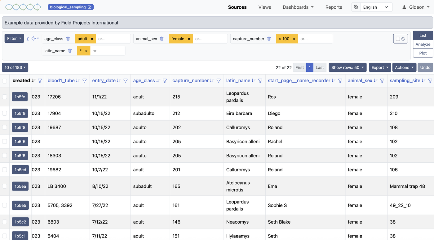
Filtering

The filter system ranges from simple to complex depending on your needs. At its simplest, you select a field and a value to match. You can stack multiple filters — they combine with AND logic, so records must satisfy all conditions to appear.

For more precise matching, filters accept regular expressions, allowing pattern-based searches across text fields. This is useful for finding values with a shared prefix, a specific format, or a range of codes.

Default filters can be saved on a source or view so that specific conditions are always active when you open it — for example, automatically showing only records from the current field season. These are set in the source or view configuration, and users can add further filters on top of them during a session.

Creating a Source

There are three distinct ways a source is created in ISLdata. Understanding the difference helps you choose the right approach for your situation.

1. Manual field-by-field setup

Navigate to Sources and click New Source. After naming the source, you add each field one at a time — specifying the name, type, and options for each. This gives you the most control over the structure and is a good choice when you're designing a collection from scratch, such as a species reference table or a sample registration form.

2. Import-driven setup

Create a blank source and immediately import a spreadsheet (CSV or XLSX). The column headers in your file become the field definitions — names, order, and all. This is the fastest way to bring an existing dataset into ISLdata and have the source structure mirror your spreadsheet automatically.

3. Automatic creation from a data collection service

If your workspace is integrated with ODK Central or ESRI Survey123, sources are created automatically — no action required. When submissions arrive from the server, ISLdata creates the source if it doesn't exist yet, establishes all the fields from the form definition, and populates the initial records. New submissions continue to sync on an ongoing basis.

Editing Source Configuration

Each source has a configuration page where you can manage its fields and their options. To access it, open the source and click the Edit button (or gear icon).

Field Aliases (Display Names)

Field names inherited from ODK forms or imported files are often technical or abbreviated. You can assign an alias — a readable display name — to any field. The original field identifier is preserved internally and continues to be used for data mapping, so renaming never breaks imports or integrations. It's purely a display change.

Field Types

Each field has a type that determines how its data is stored, sorted, and used in calculations. The available types are:

Type	Description
Text	Free-form text. The default type for imported data.
Integer	Whole number values. Enables numeric sorting and aggregation functions like sum and average.
Float	Decimal number values. Use for measurements, coordinates, or any data requiring decimal precision.
Attachment	A field that holds a reference to a binary file (image, document, etc.) associated with the record.
Lookup	A field that links to a record in another source. When a user clicks a lookup value in the data table, a pop-up opens showing the full record from the connected source — without leaving the current page. This makes it easy to cross-reference related data.
Sequence	An auto-incrementing numeric field. Useful for generating unique sequential identifiers within a source.

You can change a field's type at any time, but be aware that existing data will be validated against the new type. For example, converting a text field to an integer field will flag any non-numeric values.

Field Options

Beyond the type, individual fields support additional options:

• Required — mark a field as required so that records cannot be saved without a value in that field. This is useful for enforcing data quality on key identifiers.
• Include in default view — designate a field as part of the default column layout. Fields not included here will be hidden by default but remain accessible through column visibility controls.

Field Order

You can reorder fields in the source configuration. The new order becomes the default column sequence in the data table and is preserved across future imports — incoming data is mapped by field name, not position, so reordering never causes mapping errors.

Alternative Language Labels

If your team works across languages, you can add alternative language labels to field names. This allows users to see field headers in their preferred language without changing the underlying data structure.

Importing Data

The import wizard walks you through bringing external data into a source. This is one of the most common operations in ISLdata and supports CSV and Excel (XLSX) files.

Step 1 — Upload Your File

Select the file from your computer. ISLdata will parse it and show you a preview of the columns and first few rows so you can verify it was read correctly.

Step 2 — Field Mapping

If the source already has defined fields (from a previous import or from ODK), you'll map the columns in your file to the existing fields. If this is a new source, the columns in your file will create the field structure. You can skip columns you don't want to import.

Step 3 — Staged Review

Before the data is committed, it lands in a staging area. You can review the staged records, spot-check values, and catch any issues before they enter the source. This is your safety net — nothing is final until you commit.

Step 4 — Commit

Once you're satisfied with the staged data, commit the import. The records become part of the source, and an audit event is logged recording who imported what and when.

Inline Editing

You can edit individual field values directly in the data table by clicking on a cell. This is useful for correcting data entry errors, updating status fields, or filling in missing values without leaving the main table view.

Editing Multiple Records at Once

ISLdata doesn't have a separate "bulk edit" button or mode — instead, multi-record editing works through record selection. Select multiple records using the checkboxes on each row. Once two or more records are selected, any edit you make to a field in one of those records is automatically applied to all selected records simultaneously.

This means the workflow is: select the records you want to update, edit the field value in any one of them, and the change propagates to all. You can use filters first to narrow down the visible records, then select all of them at once to target exactly the right set.

Attachments

Records can have binary files attached to them — photographs, scanned documents, PDFs, or any other file type. Attachments from ODK form submissions (like photos taken in the field) are synced automatically. You can also upload attachments manually through the record detail view.

In-App Viewer

Common file types open directly in a pop-up viewer without needing to download the file first. Images support zoom and rotation controls, and any rotation change you make in the viewer is saved — so if a field photo was captured sideways, you can correct it once and it stays corrected. PDFs open in a built-in reader where you can scroll through pages and use text search to find content within the document.

Files that can't be previewed in the browser can still be downloaded directly to your device.

Copy-To

Copy-to is the primary mechanism for moving records through a research pipeline. The core idea is that you maintain a separate source for each stage of a process — sample collection, laboratory processing, results, and so on — and use copy-to to advance records from one stage to the next. Each copy operation logs the progression and creates a traceable link between stages.

How It Works

Select one or more records in a source (or view), then trigger copy-to and select the destination source. The records are copied in, and you can optionally override specific field values as part of the copy — for example, setting a "Received date" or a "Status" field in the destination to a fixed value at the time of transfer.

The origin_id Field

Every source has a system field called origin_id. When records arrive via copy-to, this field is automatically populated with the ID of the originating record in the source it came from. The origin_id functions as a lookup — you can click it to open the origin record in a pop-up. This gives you a backward-facing link: from any stage, you can trace a record back to where it started.

Forward-Facing Links (Auto-Increment + Lookup)

You can also set up a forward-facing link — so that when you copy a record into a destination source, the origin record is automatically updated with the ID of the new record it just created. This requires two steps in setup:

1. Create an auto-increment field in the destination source (to generate a unique ID for each new record).
2. Create a lookup field in the origin source that points to that auto-increment field in the destination.

Once this is in place, the copy-to panel will show an option labelled "Link new record(s) back to [source name]:". This is enabled by default when a compatible lookup is detected. You can toggle it off if you need to copy without creating the back-link for a particular batch.

Record Operations

Duplicating Records

Individual records can be duplicated within the same source. The duplicate is created as a new record with its own ID, so you can modify it independently. You can also override specific field values during duplication.

Archiving Records

Records can be archived rather than permanently deleted. Archived records are moved to a separate collection and hidden from the default view, but can be accessed and restored by navigating to the archive view. This is the recommended approach for removing records you no longer need — it preserves the data and the audit trail.

Understanding Views

A view is a virtual window into your data. Unlike a source, a view doesn't store data itself — it references data from one or more sources and presents it according to your configuration. If the underlying source data changes, the view reflects those changes automatically.

Views have three distinct capabilities. First, they let you customise how you see data from a single source — choosing which fields to show, renaming them, reordering them, and setting default filters. Second, they let you combine data from multiple sources in two different ways (stacking or merging — described below). Third, and perhaps most distinctively, you can add entirely new fields that exist only in the view — not present in any source — to annotate, categorise, or derive information within that view's context.

Views are non-destructive — creating or modifying a view never changes the underlying source data. When you edit records through a view, the changes are written back to the originating source and logged in the audit trail.

Creating a Single-Source View

A single-source view draws from one source and lets you customize the presentation. To create one, navigate to Views and click New View, then select your source.

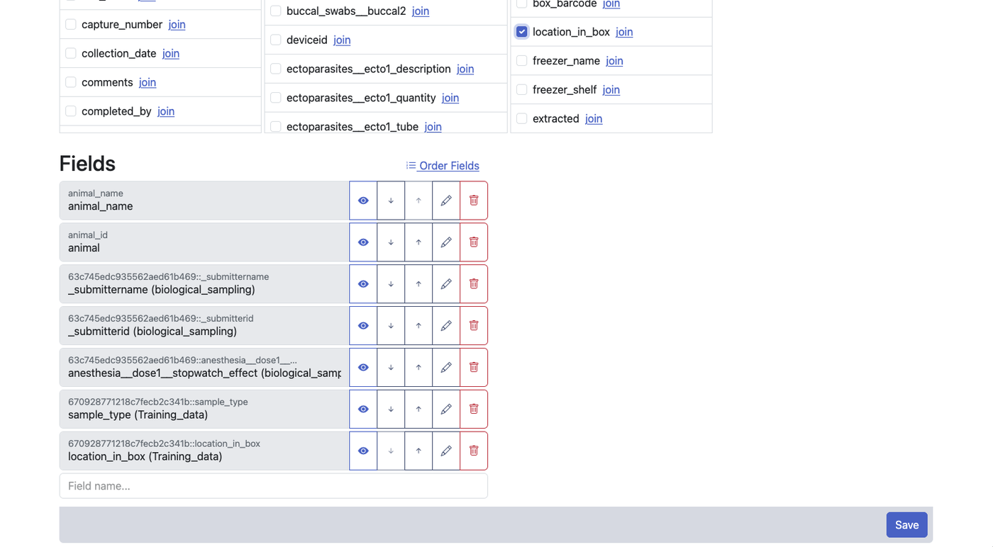
In the view builder, you can:

• Select fields — choose which source fields appear in the view. Leave out metadata or internal fields you don't need.
• Rename fields — give fields more meaningful names for this view without changing the source. For example, rename p_dob to Date of Birth.
• Reorder fields — arrange columns in a logical sequence for your workflow.
• Set default filters — pre-configure filters so the view always opens showing a specific subset of data (for example, only records from the current year).
• Set default visible columns — control which fields are visible by default when the view loads.

View-Only Fields

This is one of the most distinctive capabilities in ISLdata: you can add fields to a view that have no equivalent in any of the underlying sources. These fields exist exclusively within the view, and any data entered into them is stored there — not in the source.

This is genuinely useful when you want to work with a specific subset of your data and build a layer of interpretation or classification on top of it. For example, you might create a view of field samples and add a view-only field for a categorisation scheme that's relevant to one team's analysis, without that categorisation cluttering the original source for everyone else. The view becomes both a window and a working surface.

View-only fields are visually distinguished in the data table — highlighted to make it immediately clear that they are not sourced from the underlying data, so there's no ambiguity about where values come from.

Combining Multiple Sources

When your data lives across more than one source, ISLdata offers two fundamentally different ways to bring them together into a single view. Understanding which to use is important — they serve different analytical purposes and produce different results.

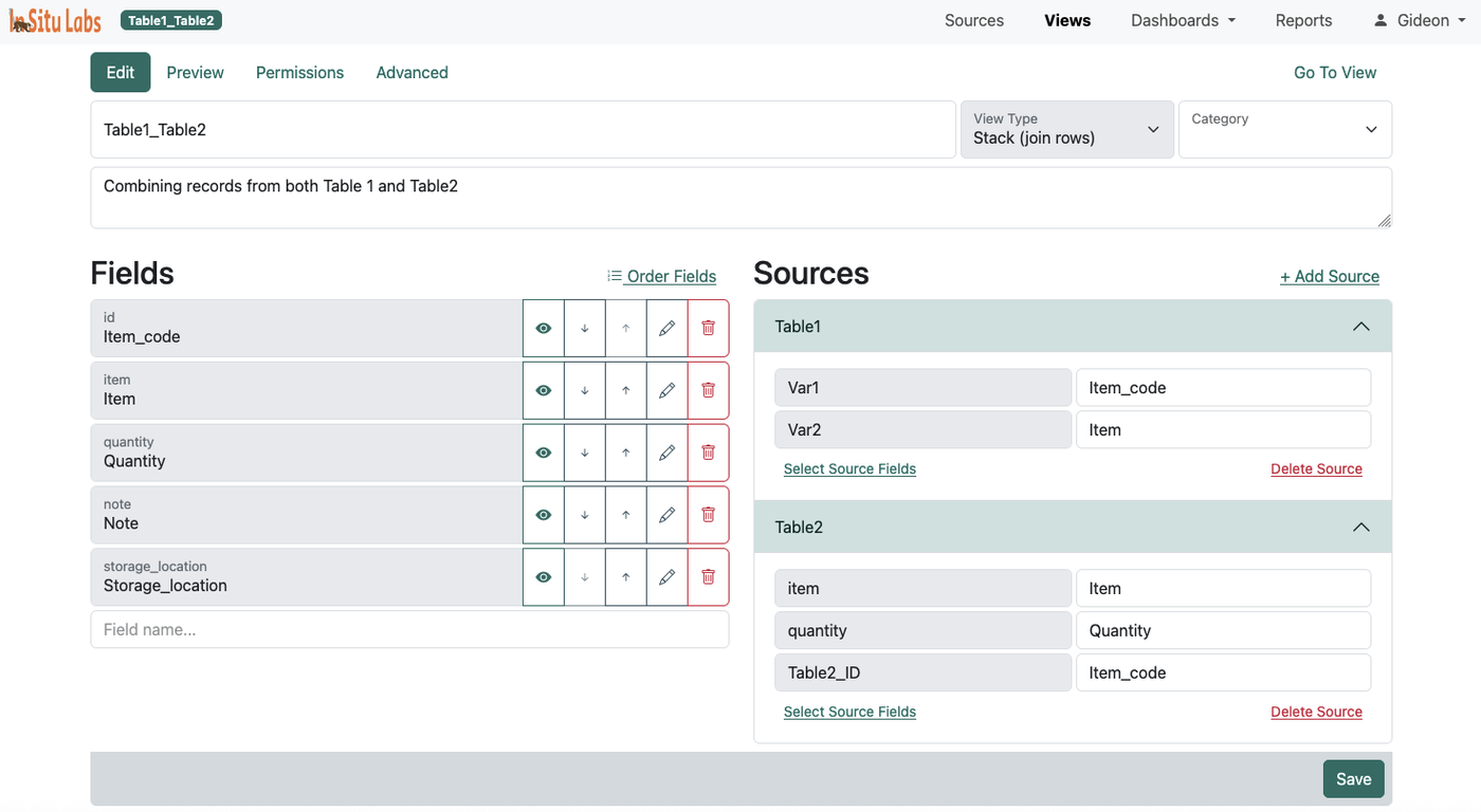
Stack Views

A stack view places records from multiple sources on top of one another into a single unified dataset. Records are not merged — they remain distinct rows. The total number of rows in a stack view equals the total number of records across all included sources combined.

To make this work, you map each source's fields to the appropriate view fields. For example, if one source calls a field collection_date and another calls the same concept sample_date, you map both to a single view field named "Date". ISLdata handles the harmonization so the data lines up correctly in the table.

Stack views are ideal when you want to co-analyse datasets that are structurally similar but separated by year, geography, project phase, or institution — situations where you want a combined picture without merging the identities of the records themselves.

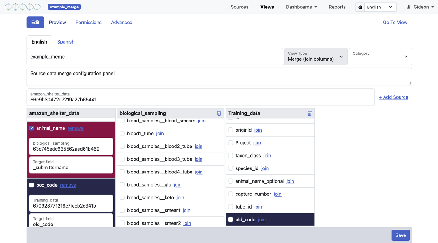
Merge Views

A merge view works more like a traditional database join. You start with one primary source and merge additional information onto each record from one or more linked sources — using a shared identifier field (equivalent to a primary/foreign key relationship) to match records across sources.

The number of rows in a merge view equals the number of records in your primary source — no more, no less. What changes is the number of columns: fields from the linked sources are appended to each record where the key field matches. To help you keep track of where each field originates, columns are colour-coded by source in the view.

A merge view is the right choice when you want to enrich a core dataset with related information — for example, combining a sample registration source with a results source, linking on a shared sample ID.

Editing Through Views

Both stack and merge views support editing. When you edit a record through a view, the change is written back to the original source — the view is just a window, not a copy. All changes made through views are recorded in the audit trail and can be undone by a user with the appropriate privileges.

A Note on Referential Integrity

Unlike a traditional relational database, ISLdata does not enforce referential integrity between linked sources. This is intentional — strict enforcement often creates obstacles in research data workflows where data arrives incrementally and imperfectly. You can achieve similar safeguards by using lookup fields to establish relationships between sources and marking critical linking fields as required. This gives you the flexibility of a document-based system with the organisational discipline of relational design, applied where it matters most.

Materialized Views

When a view is complex — combining large sources, involving multiple joins, or doing heavy aggregation — querying it live on every page load can be slow. Materialized views solve this by pre-computing and caching the view's result in the background, so the data loads instantly when you open it.

Materialized views are enabled by default for views where the system detects they would help. The cache is refreshed automatically whenever the system detects a change to the view's definition or its underlying sources, and also on a regular schedule. Workspace administrators can also trigger a manual refresh at any time if they need the view to reflect very recent changes immediately.

Reduce & Group

The Analyze function is available on any source or view. It lets you summarise your data by grouping records on one or more fields and applying a calculation across each group — similar to a pivot table in a spreadsheet, but built directly into the data viewer.

How to Use It

Click the Analyze button on any source or view. A panel will open where you:

1. Select one or more grouping variables — the fields whose distinct values define the groups (e.g. Site, Species, Month).
2. Choose the operation to perform: count, sum, average, minimum, or maximum.
3. Select the field the operation should be applied to.

The result is a summary table showing one row per group with the calculated value. You can apply multiple grouping variables to produce cross-tabulations — for example, grouping by both site and year to see counts broken down across both dimensions.

Summary tables can be exported directly (see Exporting Data) or added to a report for inclusion in a formatted document.

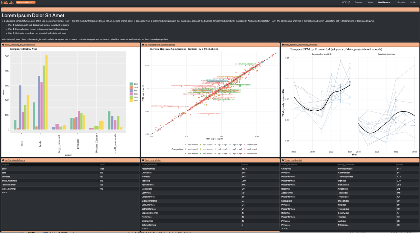
Dashboards

A dashboard is a page of widgets that brings together multiple views of your data in one place. Dashboards are useful for monitoring data collection progress, tracking key metrics at a glance, or sharing a live summary with collaborators. Widgets can display:

• Charts and plots — saved visualizations from any source or view
• Data summaries — aggregated or reduced views of your data
• Record lists — live tables of records drawn from a source or view
• Rich text blocks — headings, explanatory notes, or context for other viewers

Building a Dashboard

Navigate to Dashboards and create a new one. From the dashboard editor you can add any of the widget types above, arrange them on the page, and configure each widget's data source and filters individually.

You don't have to build everything from the dashboard editor. From within any source or view, you can send a plot or summary directly to an existing dashboard — or create a new one on the spot. This makes it easy to build up a dashboard incrementally as you're working through your data, rather than having to switch contexts.

Reports

Reports are structured documents that mix narrative writing with live data content. They're designed for writing up findings, producing periodic summaries, or sharing results with people who need more context than a dashboard provides.

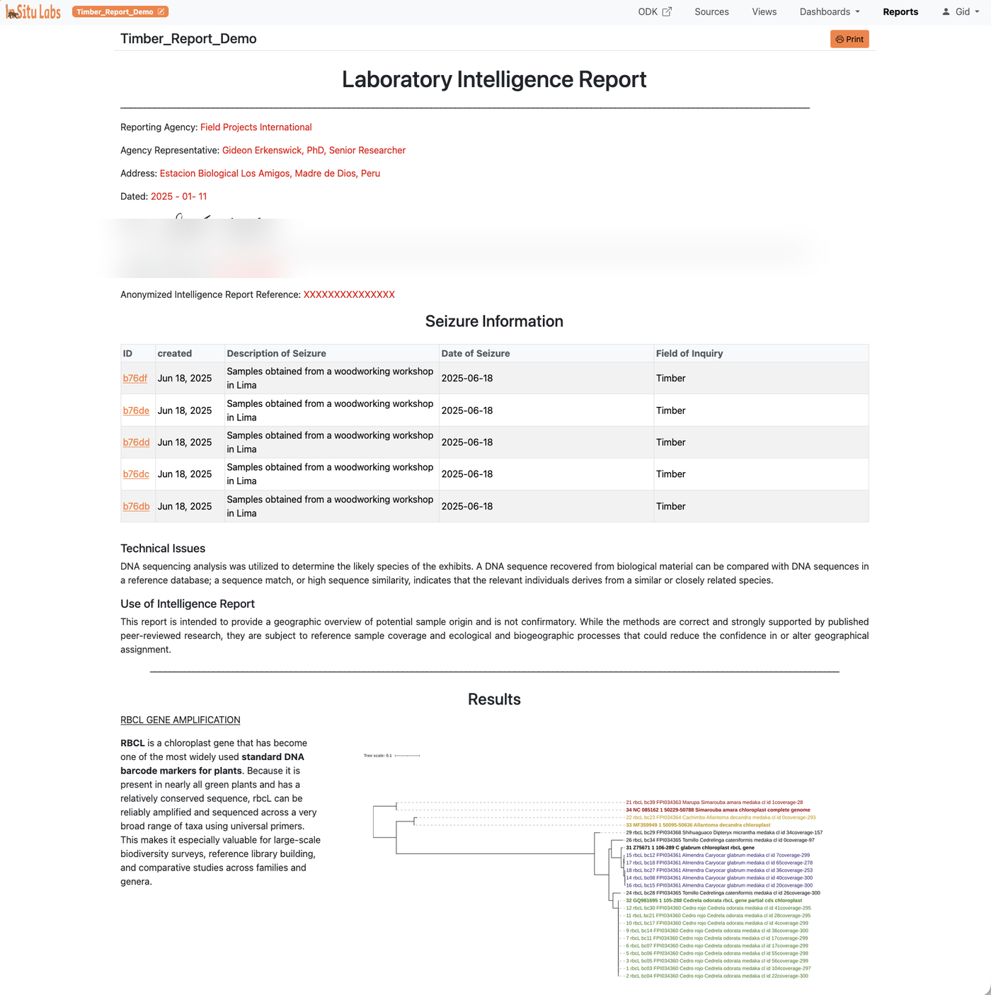
What You Can Embed

A report can contain any combination of the following, in any order:

• Saved plots from any source or view
• Data summaries and aggregations from any source or view
• Record lists drawn from any source or view
• External images — uploaded or linked from a URL
• Hyperlinks — to external resources or other parts of the system
• Rich text — headings, body paragraphs, captions, and formatted narrative

Live Record Links

Records listed within a report are live links. Clicking a record opens it directly in the data system — provided you have permission to access the source it belongs to. This makes reports useful not just as summaries but as navigation tools, letting readers drill into any individual record that catches their attention.

Exporting

Reports can be exported as PDF (via print) or shared as HTML. The formatting is designed to produce clean, professional output suitable for sending to collaborators, funders, or institutional partners who don't have access to the system.

Plots & Visualizations

Plots are the building blocks of dashboards and reports — charts, graphs, and any other visual representation of your data. They're created using R code, giving you the full flexibility of R's graphics ecosystem for any visualization you need.

Creating a Plot

Open any source or view and select the Plot tab. This opens a code workspace where you write R code to generate your visualization. Your data is automatically available as an R data.frame called data — no loading or setup required.

To render your plot, press Ctrl+Enter (Windows/Linux) or Cmd+Enter (Mac), or click the Render button. The output appears immediately alongside your code.

Example

Here's a simple bar chart using base R — replace field names with your own:

barplot(
  table(data$species),
  main = "Records by Species",
  xlab = "Species",
  ylab = "Count",
  col  = "steelblue"
)

For more complex plots, the same pattern applies — write or paste in any R plotting code that operates on data and outputs a graphic.

Using AI Tools to Help Write Plots

Because the data is a standard R data.frame, you can use any external AI tool to help write plotting code. To give the AI the context it needs, run str(data) in the workspace — this prints a summary of the data structure (field names, types, and sample values). Copy that output into your AI tool alongside your plot request, and the AI will be able to write code that references your actual field names correctly.

Saving and Sharing Plots

Once a plot looks the way you want, save it. Saved plots can be added to any dashboard or report from the dashboard editor or report editor — or sent directly to an existing dashboard from within the source or view you're working in.

Plots are rendered as SVG graphics, so they scale cleanly at any size and look sharp when exported to PDF.

Filters and the data Object

Whatever filters are active on the source or view when you open the Plot tab are already reflected in the data object — you're always working with the filtered dataset, not the full one. This gives you two ways to control what goes into a plot:

• Hardcode filters in R — write filtering logic directly into your plot code using standard R (e.g. data[data$site == "Site-A", ]). This makes the filter permanent and explicit within the code itself.
• Use the system's filter tools — apply filters through ISLdata's filtering interface before opening the Plot tab. The code stays clean and general, and the filter is controlled externally.

When you save a plot, you have the option to save with the current filters or save without filters. Saving without hardcoded filters is often the more flexible choice — it means you can tweak the active filters using the system's tools and re-render the same plot instantly to see how it changes. This is particularly useful when you're iterating across subsets: adjusting by year, site, or species and updating the visualisation rapidly without touching the code.

Available R Packages

The plotting environment runs in a pre-configured Docker container with a wide range of common R packages for data manipulation and visualisation already installed. If you need a package that isn't available, contact support to have it added to the environment. If you're self-hosting ISLdata, you have full control over the Docker container and can add any packages you need directly.

Exporting Data

You can export data from any source or view as a CSV or Excel (XLSX) file. This works identically whether you're in a source or a view — the export always reflects exactly what you're looking at: the currently visible fields, in the current column order, with any active filters applied. What you see is what you get.

Field names in the export match what you see on screen — including any aliases assigned in source configuration and any renames applied in views. This means your exported file is immediately readable without needing to decode internal field IDs.

Reduce & Group summaries (see Reduce & Group) can also be exported from the Analyze panel in the same way.

Permissions & Sharing

Access control in ISLdata applies to every object in the system — sources, views, dashboards, and reports each have their own independent permission settings. This means you can grant a user access to a curated view of data without giving them access to the underlying source, or share a dashboard publicly while keeping the source it draws from private.

How Permissions Work

Permissions are set per-user and per-object. There are two levels:

• Read — the user can see the object and its data, but cannot make changes.
• Write — the user can read and edit data within the object (adding, modifying, or removing records where applicable).

Workspace administrators bypass all permission checks — they have full access to everything in the workspace by default. For all other users, only objects they have been explicitly granted access to will appear in their navigation.

Object	Read grants	Write grants
Source	Browse records, filter, export	Also: add, edit, import, and archive records
View	Browse and export view data	Also: edit records through the view (writes back to source)
Dashboard	View the dashboard	Also: edit layout and widget configuration
Report	View and read the report	Also: edit report content and structure

Logging In

ISLdata uses passwordless authentication. There's no password to create, remember, or reset. Here's how it works:

1. Navigate to your ISLdata instance and enter your email address.
2. Check your inbox — you'll receive an email with a secure login link.
3. Click the link. You're now logged in and your session is established.

The login link is single-use and time-limited for security. If it expires, simply request a new one. You need access to a secure email account — this is your authentication factor instead of a password.

Preferences & Organisation

Your user preferences include theme selection and default display settings. These are stored per-user and don't affect other users in the workspace.

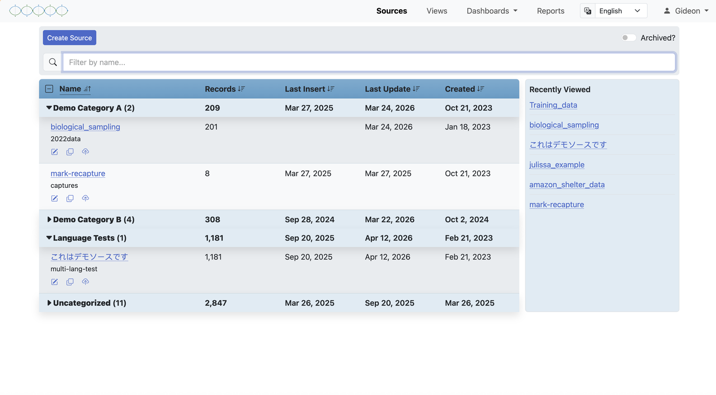
Categories

As a workspace grows, the lists of sources, views, reports, and dashboards can become long. Categories let you assign any of these objects to a named group, giving your workspace structure and reducing clutter in the navigation panels.

Categories are created and managed from within the relevant panel — sources, views, reports — and any object can be assigned to one. Once categories are in place, they act as a way to browse by project, phase, dataset type, or however your team thinks about its work.

If you're looking for something specific, every panel also has a search bar that lets you find any source, view, report, or dashboard by name directly — useful when you know what you're after and don't want to browse through categories.

Understanding Your Permissions

Your access to specific sources, views, dashboards, and reports is controlled by the permissions assigned to you by a workspace administrator. You'll only see items you have access to in the sidebar navigation.

If you need access to a source or view you can't see, contact your workspace administrator. They can grant you read access (to view the data) or write access (to edit records) on a per-resource basis.

Role	What You Can Do
Workspace Member	Access sources, views, dashboards, and reports you've been granted permission to. Export data. Edit records in sources/views where you have write access.
Workspace Admin	Everything a member can do, plus: manage users, set permissions, view the full audit log, create and configure all resources.